
Under ICLR 2024 double-blind review
使用一个自动编码器,来提取训练模型参数中的隐藏表征,然后扩散模型根据这些隐藏参数表征,合成一些随机噪声,输出一些新的表征给自动编码器的解码器部分,输出就是神经网络的参数。
神经网络扩散
初步了解扩散模型
扩散模型分为两个过程,前向过程和反向过程:
前向过程是对原始图像不断添加高斯噪声(由$\beta$约束),经过$T$步后,得到一个随机高斯噪声($T\to \infty$时,最后得到的一定是噪声)
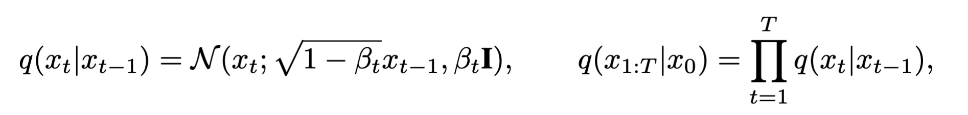
- $q(.)$:前向过程
- $N(.)$:高斯噪声
- $\beta$:约束
- $I$:单位矩阵
反向过程是前向过程反过来,期望通过选连一个去噪网络(denoising network),移除掉$x_T$上的噪声,直到恢复出原始图像来。

- $p_\theta (.)$:反向过程,$\theta$是可学习的参数
- $\mu _\theta (.)$:通过$\theta$估计的高斯噪声的均值
- $\sum _\theta (.)$:通过$\theta$估计的高斯噪声的方差
去噪网络的优化:
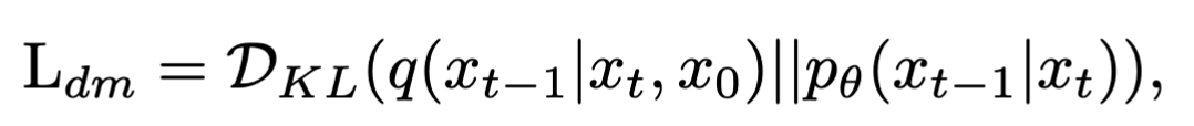
$D_{KL}(.\vert \vert .)$是通过KL散度来计算两个分布之间的差距。
扩散模型的可行之处在于:能够通过反向过程找到一个去噪网络,将原始的高斯分布转化成最终期望得到的分布。
整体架构
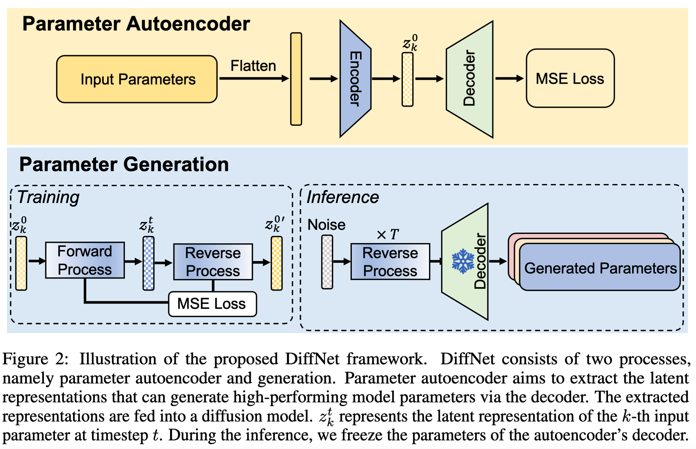
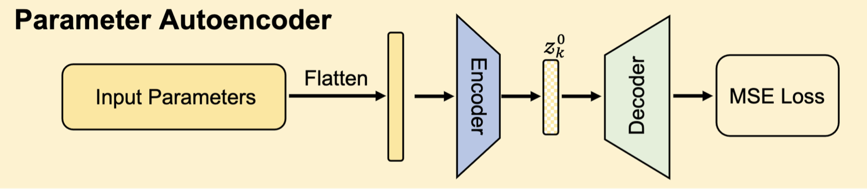
参数自动编码器
首先收集k个训练性能良好的模型,其参数可以表示为:$S=[s_1,…,s_K]$,将这些参数展开平铺成向量:$V=[v_1,…v_K]$,然后通过编码器来提取参数潜在的特征:
$$
Z=[z_1,…,z_K]=f_{encoder}(V,\sigma)
$$
然后将提取出的潜在参数特征$Z$输入到解码器中生成重构后的参数:
$$
V^{‘}=[v_1^{‘},…,v_K^{‘}]=f_{decoder}(Z,\rho)
$$
其中$\sigma,\rho$是参数。
优化路径是最小化MSE:
$$
L_{MSE}=\frac{1}{K}\sum _1^K\Vert v _k-v_k^{‘}\Vert^2
$$
参数生成
若是直接采取将参数$V$输入到编码器,然后解码器输出重构后的参数$V_{‘}$,这样会导致过大的存储开销,尤其是当$V$的维度比较高的时候。
因此,作者采用DDPM中的优化过程来优化去噪网络;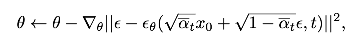
- $\epsilon$:高斯噪声
- $\theta$:去噪网络的参数
- $\epsilon _\theta$:去噪网络生成的噪声
- $t$:每一轮
- $\bar \alpha _t$:每一轮的噪声强度
实验
设置
数据集
MNIST (LeCun et al., 1998), CIFAR-10/100 (Krizhevsky et al., 2009), ImageNet-1K. (Deng et al., 2009), STL-10 (Coates et al., 2011), Flowers (Nilsback & Zisserman, 2008), Pets (Parkhi et al., 2012), F-101 (Bossard et al., 2014)
架构
最开始是在比较小的模型上实验的,这些模型由卷积层、池化层、全连接层组成:
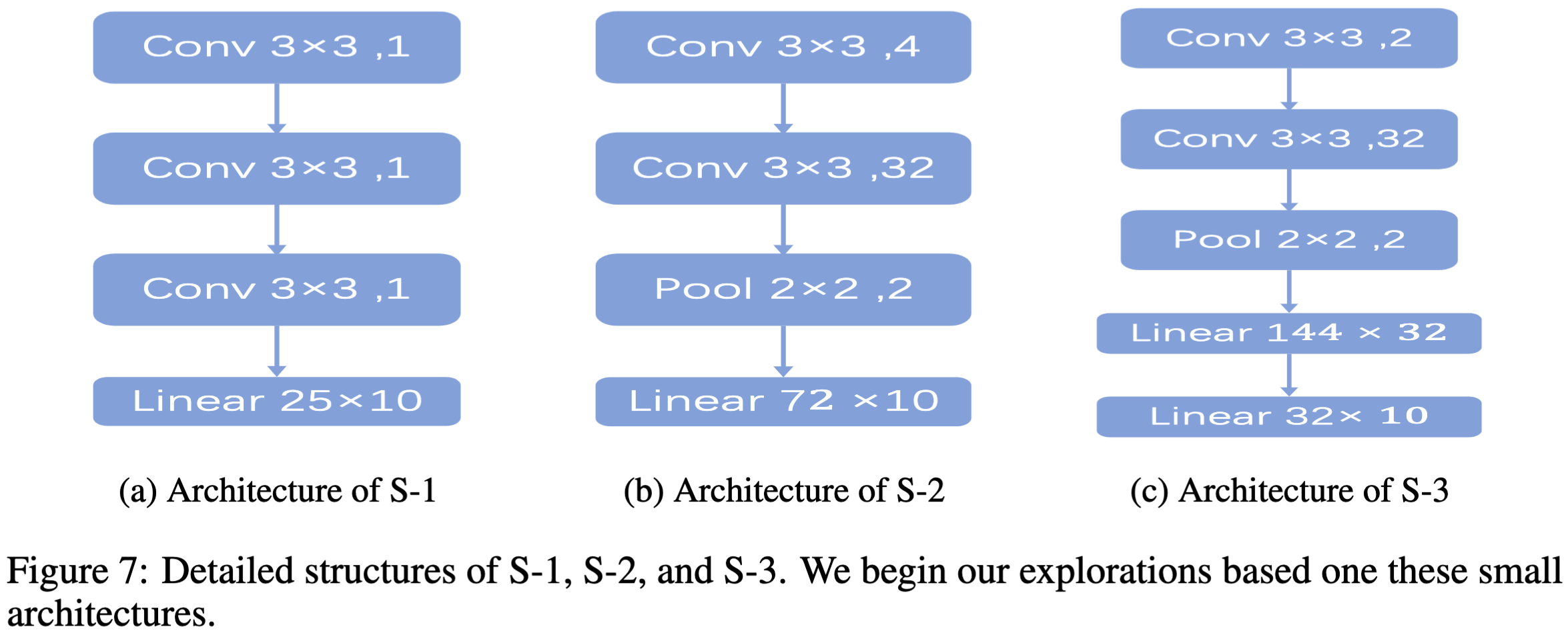
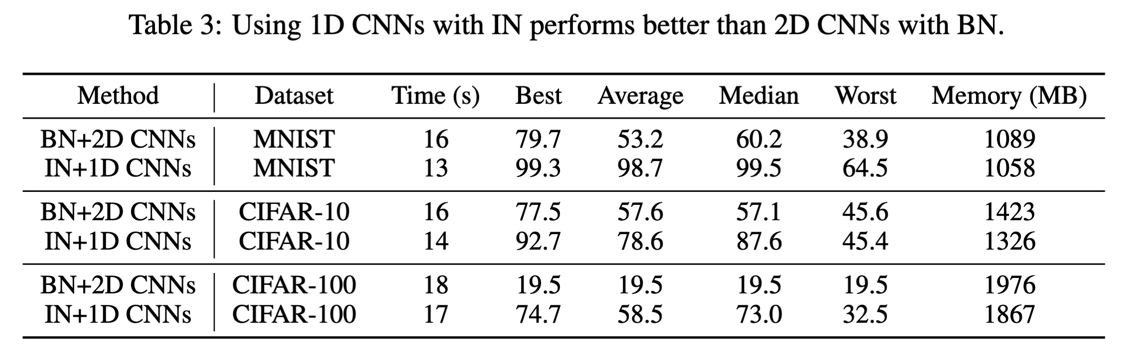
使用的卷积层是2D卷积,参考的是DDPM(采用的U-net,生成高质量图片,用的2D-conv),但是效果并不好,可能的原因是图片像素和参数不能一概处理,因此换成了1D-conv,对比结果如下:
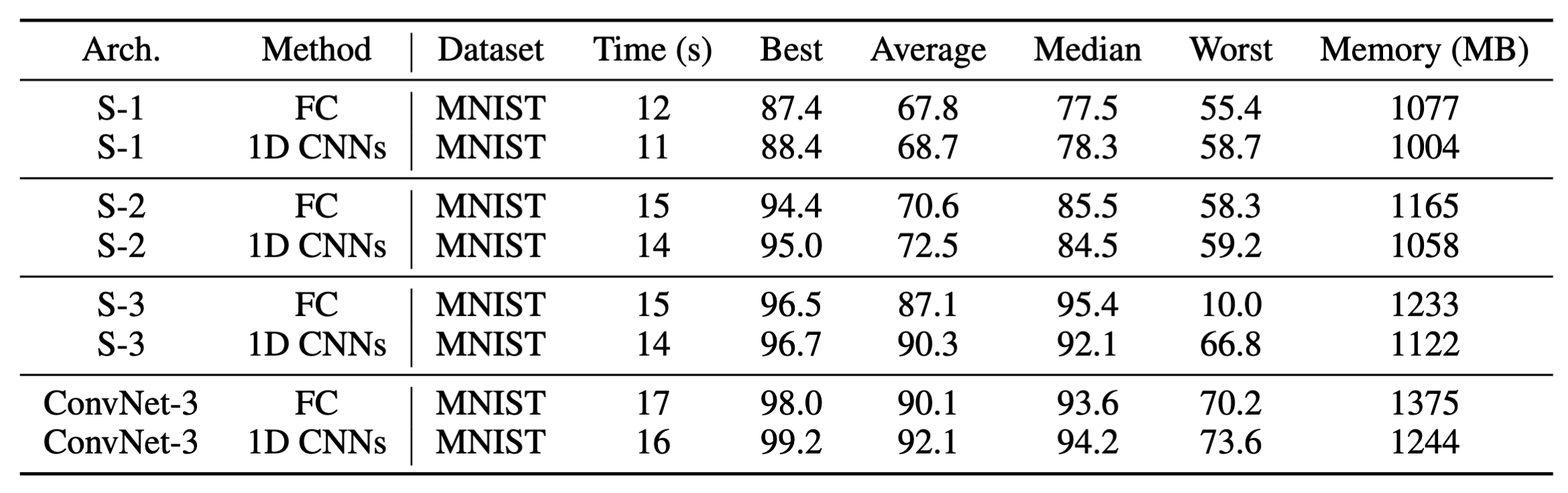
在更换卷积层的时候,作者也考虑了下直接将卷积层更换为FC,二者效果差不多,但是1D-conv的存储开销低于FC,因此还是选取了1D-conv:
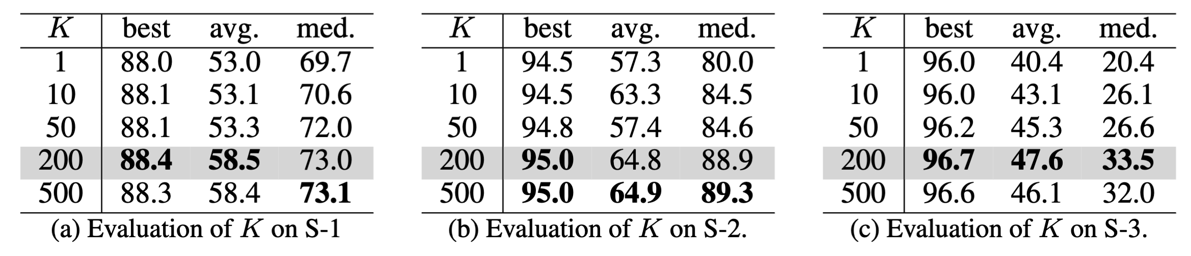
此外,还做了消融实验,找到了一个参数$K=200$使得模型的性能最优。
作者是在扩大模型架构的时候发现了存储开销特别大的问题,灵感来于stable diffusion,作者采用了一个自动编码器来提取潜在特征,以此来对模型的参数进行降维。
准备训练数据
准备了200个独立的高性能参数来训练DiffNet,对于架构简单,参数少的模型,直接从头开始训练;对于架构复杂的,则是在预训练模型的基础上来进行的。
训练细节
首先把自动编码器训练2000轮,然后将潜在特征和解码器的参数都保存起来。
然后训练扩散模型来生成表征,扩散模型的结构式基于1D-conv的U-Net,
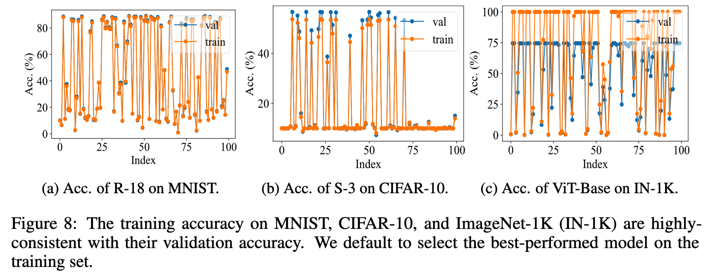
推断阶段
将100个噪声输入到扩散模型中去,生成了100个模型,选取其中在训练数据集上性能最好的网络。整个的性能图如下:
代码阅读
准备训练数据
作者通过训练一个ResNet18来得到编码器的训练数据。,也就是下图中的参数输入部分:
代码部分在tsak_training.py中,核心部分是这个:
1 | # override the abstract method in base_task.py, you obtain the model data for generation |
训练一共有400轮:
首先将ResNet18训练200轮,将其参数保存下来:
1
2
3
4
5
6
7if i == (epoch - 1):
# 在第199的时候保存模型
print("saving the model")
torch.save(net, os.path.join(tmp_path, "whole_model.pth"))
# 将不需要训练的层进行固定(取消梯度),后续训练只训练需要训练的层train_layer
fix_partial_model(train_layer, net)
parameters = []在200轮后的训练中,只训练需要需要训练的层,其他的层的参数被冻结了,每过10轮,都会将训练的层的参数保存下来,存储到临时文件夹中。
1
2
3
4
5
6
7
8
9if i >= epoch:
# 在接下来的训练中,每训练一轮,都会将需要保存的层的参数保存下来,存储到一个列表中
parameters.append(state_part(train_layer, net))
save_model_accs.append(acc)
# 当列表的长度等于10时,或者到达训练结束的时候,将参数保存在硬盘上的临时文件夹中。
if len(parameters) == 10 or i == all_epoch - 1:
torch.save(parameters, os.path.join(tmp_path, "p_data_{}.pt".format(i)))
# 初始化列表
parameters = []最后得到了一个最重要的数据
data.pt,里面存储了整个模型whole_model.pth,编码器需要的训练数据pdata,可以将data.ptload一下: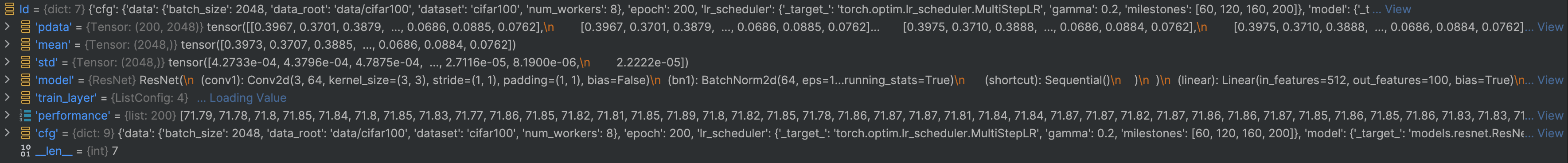
1
2
3
4
5
6
7
8
9
10
11
12
13
14
15
16
17
18
19
20
21
22
23
24
25
26
27
28
29
30
31
32
33
34
35
36
37
38
39
40
41
42
43
44
45
46
47
48
49
50
51
52
53
54
55
56
57
58
59
60
61
62
63
64
65
66
67
68
69
70
71
72
73
74
75
76
77
78
79
80
81
82
83
84
85
86
87
88
89
90
91
92
93
94
95
96
97
98
99
100
101
102
103
104{'pdata': tensor([[0.3967, 0.3701, 0.3879, ..., 0.0686, 0.0885, 0.0762],
[0.3967, 0.3701, 0.3879, ..., 0.0686, 0.0885, 0.0762],
[0.3967, 0.3701, 0.3878, ..., 0.0686, 0.0885, 0.0762],
...,
[0.3975, 0.3710, 0.3888, ..., 0.0686, 0.0884, 0.0762],
[0.3975, 0.3710, 0.3888, ..., 0.0686, 0.0884, 0.0762],
[0.3975, 0.3710, 0.3888, ..., 0.0686, 0.0884, 0.0762]]), 'mean': tensor([0.3973, 0.3707, 0.3885, ..., 0.0686, 0.0884, 0.0762]), 'std': tensor([4.2733e-04, 4.3796e-04, 4.7875e-04, ..., 2.7116e-05, 8.1900e-06,
2.2222e-05]), 'model': ResNet(
(conv1): Conv2d(3, 64, kernel_size=(3, 3), stride=(1, 1), padding=(1, 1), bias=False)
(bn1): BatchNorm2d(64, eps=1e-05, momentum=0.1, affine=True, track_running_stats=True)
(layer1): Sequential(
(0): BasicBlock(
(conv1): Conv2d(64, 64, kernel_size=(3, 3), stride=(1, 1), padding=(1, 1), bias=False)
(bn1): BatchNorm2d(64, eps=1e-05, momentum=0.1, affine=True, track_running_stats=True)
(conv2): Conv2d(64, 64, kernel_size=(3, 3), stride=(1, 1), padding=(1, 1), bias=False)
(bn2): BatchNorm2d(64, eps=1e-05, momentum=0.1, affine=True, track_running_stats=True)
(shortcut): Sequential()
)
(1): BasicBlock(
(conv1): Conv2d(64, 64, kernel_size=(3, 3), stride=(1, 1), padding=(1, 1), bias=False)
(bn1): BatchNorm2d(64, eps=1e-05, momentum=0.1, affine=True, track_running_stats=True)
(conv2): Conv2d(64, 64, kernel_size=(3, 3), stride=(1, 1), padding=(1, 1), bias=False)
(bn2): BatchNorm2d(64, eps=1e-05, momentum=0.1, affine=True, track_running_stats=True)
(shortcut): Sequential()
)
)
(layer2): Sequential(
(0): BasicBlock(
(conv1): Conv2d(64, 128, kernel_size=(3, 3), stride=(2, 2), padding=(1, 1), bias=False)
(bn1): BatchNorm2d(128, eps=1e-05, momentum=0.1, affine=True, track_running_stats=True)
(conv2): Conv2d(128, 128, kernel_size=(3, 3), stride=(1, 1), padding=(1, 1), bias=False)
(bn2): BatchNorm2d(128, eps=1e-05, momentum=0.1, affine=True, track_running_stats=True)
(shortcut): Sequential(
(0): Conv2d(64, 128, kernel_size=(1, 1), stride=(2, 2), bias=False)
(1): BatchNorm2d(128, eps=1e-05, momentum=0.1, affine=True, track_running_stats=True)
)
)
(1): BasicBlock(
(conv1): Conv2d(128, 128, kernel_size=(3, 3), stride=(1, 1), padding=(1, 1), bias=False)
(bn1): BatchNorm2d(128, eps=1e-05, momentum=0.1, affine=True, track_running_stats=True)
(conv2): Conv2d(128, 128, kernel_size=(3, 3), stride=(1, 1), padding=(1, 1), bias=False)
(bn2): BatchNorm2d(128, eps=1e-05, momentum=0.1, affine=True, track_running_stats=True)
(shortcut): Sequential()
)
)
(layer3): Sequential(
(0): BasicBlock(
(conv1): Conv2d(128, 256, kernel_size=(3, 3), stride=(2, 2), padding=(1, 1), bias=False)
(bn1): BatchNorm2d(256, eps=1e-05, momentum=0.1, affine=True, track_running_stats=True)
(conv2): Conv2d(256, 256, kernel_size=(3, 3), stride=(1, 1), padding=(1, 1), bias=False)
(bn2): BatchNorm2d(256, eps=1e-05, momentum=0.1, affine=True, track_running_stats=True)
(shortcut): Sequential(
(0): Conv2d(128, 256, kernel_size=(1, 1), stride=(2, 2), bias=False)
(1): BatchNorm2d(256, eps=1e-05, momentum=0.1, affine=True, track_running_stats=True)
)
)
(1): BasicBlock(
(conv1): Conv2d(256, 256, kernel_size=(3, 3), stride=(1, 1), padding=(1, 1), bias=False)
(bn1): BatchNorm2d(256, eps=1e-05, momentum=0.1, affine=True, track_running_stats=True)
(conv2): Conv2d(256, 256, kernel_size=(3, 3), stride=(1, 1), padding=(1, 1), bias=False)
(bn2): BatchNorm2d(256, eps=1e-05, momentum=0.1, affine=True, track_running_stats=True)
(shortcut): Sequential()
)
)
(layer4): Sequential(
(0): BasicBlock(
(conv1): Conv2d(256, 512, kernel_size=(3, 3), stride=(2, 2), padding=(1, 1), bias=False)
(bn1): BatchNorm2d(512, eps=1e-05, momentum=0.1, affine=True, track_running_stats=True)
(conv2): Conv2d(512, 512, kernel_size=(3, 3), stride=(1, 1), padding=(1, 1), bias=False)
(bn2): BatchNorm2d(512, eps=1e-05, momentum=0.1, affine=True, track_running_stats=True)
(shortcut): Sequential(
(0): Conv2d(256, 512, kernel_size=(1, 1), stride=(2, 2), bias=False)
(1): BatchNorm2d(512, eps=1e-05, momentum=0.1, affine=True, track_running_stats=True)
)
)
(1): BasicBlock(
(conv1): Conv2d(512, 512, kernel_size=(3, 3), stride=(1, 1), padding=(1, 1), bias=False)
(bn1): BatchNorm2d(512, eps=1e-05, momentum=0.1, affine=True, track_running_stats=True)
(conv2): Conv2d(512, 512, kernel_size=(3, 3), stride=(1, 1), padding=(1, 1), bias=False)
(bn2): BatchNorm2d(512, eps=1e-05, momentum=0.1, affine=True, track_running_stats=True)
(shortcut): Sequential()
)
)
(linear): Linear(in_features=512, out_features=100, bias=True)
), 'train_layer': ['layer4.1.bn1.weight', 'layer4.1.bn1.bias', 'layer4.1.bn2.bias', 'layer4.1.bn2.weight'], 'performance': [71.79, 71.78, 71.8, 71.85, 71.84, 71.8, 71.85, 71.83, 71.77, 71.86, 71.85, 71.82, 71.81, 71.85, 71.89, 71.8, 71.82, 71.85, 71.78, 71.86, 71.87, 71.87, 71.81, 71.84, 71.84, 71.87, 71.87, 71.82, 71.87, 71.86, 71.86, 71.87, 71.85, 71.86, 71.85, 71.86, 71.83, 71.83, 71.93, 71.91, 71.84, 71.8, 71.88, 71.84, 71.78, 71.81, 71.82, 71.8, 71.84, 71.83, 71.85, 71.85, 71.89, 71.75, 71.84, 71.78, 71.82, 71.9, 71.86, 71.89, 71.81, 71.8, 71.84, 71.86, 71.81, 71.84, 71.86, 71.82, 71.84, 71.76, 71.83, 71.82, 71.87, 71.86, 71.83, 71.87, 71.84, 71.81, 71.85, 71.84, 71.87, 71.76, 71.85, 71.78, 71.75, 71.86, 71.88, 71.83, 71.85, 71.83, 71.86, 71.86, 71.85, 71.85, 71.9, 71.86, 71.84, 71.87, 71.88, 71.86, 71.82, 71.82, 71.84, 71.84, 71.82, 71.89, 71.79, 71.86, 71.84, 71.8, 71.86, 71.85, 71.83, 71.83, 71.84, 71.89, 71.87, 71.86, 71.8, 71.84, 71.83, 71.79, 71.84, 71.9, 71.85, 71.86, 71.88, 71.84, 71.86, 71.86, 71.84, 71.86, 71.78, 71.83, 71.87, 71.89, 71.81, 71.86, 71.77, 71.84, 71.92, 71.82, 71.81, 71.8, 71.78, 71.85, 71.89, 71.81, 71.75, 71.8, 71.81, 71.84, 71.88, 71.8, 71.85, 71.8, 71.85, 71.8, 71.95, 71.85, 71.87, 71.83, 71.87, 71.84, 71.82, 71.87, 71.8, 71.86, 71.81, 71.89, 71.86, 71.84, 71.87, 71.81, 71.87, 71.83, 71.82, 71.88, 71.85, 71.84, 71.79, 71.84, 71.81, 71.84, 71.86, 71.85, 71.85, 71.85, 71.83, 71.81, 71.87, 71.83, 71.88, 71.84, 71.85, 71.81, 71.81, 71.76, 71.89, 71.86], 'cfg': {'name': 'classification', 'data': {'data_root': 'data/cifar100', 'dataset': 'cifar100', 'batch_size': 2048, 'num_workers': 8}, 'model': {'_target_': 'models.resnet.ResNet18', 'num_classes': 100}, 'optimizer': {'_target_': 'torch.optim.SGD', 'lr': 0.1, 'momentum': 0.9, 'weight_decay': 0.0005}, 'lr_scheduler': {'_target_': 'torch.optim.lr_scheduler.MultiStepLR', 'milestones': [60, 120, 160, 200], 'gamma': 0.2}, 'epoch': 200, 'save_num_model': 200, 'train_layer': ['layer4.1.bn1.weight', 'layer4.1.bn1.bias', 'layer4.1.bn2.bias', 'layer4.1.bn2.weight'], 'param': {'data_root': 'param_data/cifar100/data.pt', 'k': 200, 'num_workers': 4}}}
### 训练扩散模型
代码`train_p_diff.py`,有两种模式,可以在`base.yaml`中选择是训练或者是测试扩散模型。
项目作者将代码封装的比较好,核心代码在`core`文件夹里面。
## 实验结果
再次梳理一下这篇论文对应的实验的思路:数据集设置为CIFAR10,网络为ResNet18
1. 在CIFAR10上训练ResNet18,将得到的模型保存下来,在test_data上进行测试,得到acc:
```shell
/home/chengyiqiu/miniconda3/envs/pdiff/bin/python /home/chengyiqiu/code/diffusion/Diffuse-Backdoor-Parameters/test.py
10.0 # 这是随机初始化ResNet的acc,十类瞎猜理论上是1/10
86.034 # 这是加载了保存的state_dict后的ResNet18的准确率,良好
Process finished with exit code 0将训练好的ResNet18,选取train-layer,只训练这些层,其他的层的参数冻结(require grad = false),然后训练200个epoch,将train-layer的参数收集起来,假设模型的train-layer的长度是5120,那么收集到的数据的shape就是:(200, 5120),通过这些数据训练一个扩散模型。
用训练好的扩散模型生成参数,输入的噪声的维度是(200, latent_shape),得到200个生成的train-layer的参数,将其加入到第二步中最开始训练好的ResNet18中,替换对应层的参数,并进行测试,下面是测试结果:
这是不替换对应层参数的结果:
1
# model = partial_reverse_tomodel(param, model, train_layer).to(param.device)
1
2
3
4
5
6
7
8
9
10
11
12
13
/home/chengyiqiu/miniconda3/envs/pdiff/bin/python /home/chengyiqiu/code/diffusion/Diffuse-Backdoor-Parameters/outputs/cifar10/ae_ddpm_cifar10_pth/load.py
/home/chengyiqiu/miniconda3/envs/pdiff/lib/python3.8/site-packages/torch/nn/modules/instancenorm.py:80: UserWarning: input's size at dim=1 does not match num_features. You can silence this warning by not passing in num_features, which is not used because affine=False
warnings.warn(f"input's size at dim={feature_dim} does not match num_features. "
ae param shape: torch.Size([200, 7178])
Files already downloaded and verified
| | 0/200 [00:00<?, ?it/s]/home/chengyiqiu/miniconda3/envs/pdiff/lib/python3.8/site-packages/torch/nn/_reduction.py:42: UserWarning: size_average and reduce args will be deprecated, please use reduction='sum' instead.
warnings.warn(warning.format(ret))
|██████████| 200/200 [04:04<00:00, 1.22s/it]
Sorted list of accuracies: [92.67, 92.67, 92.67, 92.67, 92.67, 92.67, 92.67, 92.67, 92.67, 92.67, 92.67, 92.67, 92.67, 92.67, 92.67, 92.67, 92.67, 92.67, 92.67, 92.67, 92.67, 92.67, 92.67, 92.67, 92.67, 92.67, 92.67, 92.67, 92.67, 92.67, 92.67, 92.67, 92.67, 92.67, 92.67, 92.67, 92.67, 92.67, 92.67, 92.67, 92.67, 92.67, 92.67, 92.67, 92.67, 92.67, 92.67, 92.67, 92.67, 92.67, 92.67, 92.67, 92.67, 92.67, 92.67, 92.67, 92.67, 92.67, 92.67, 92.67, 92.67, 92.67, 92.67, 92.67, 92.67, 92.67, 92.67, 92.67, 92.67, 92.67, 92.67, 92.67, 92.67, 92.67, 92.67, 92.67, 92.67, 92.67, 92.67, 92.67, 92.67, 92.67, 92.67, 92.67, 92.67, 92.67, 92.67, 92.67, 92.67, 92.67, 92.67, 92.67, 92.67, 92.67, 92.67, 92.67, 92.67, 92.67, 92.67, 92.67, 92.67, 92.67, 92.67, 92.67, 92.67, 92.67, 92.67, 92.67, 92.67, 92.67, 92.67, 92.67, 92.67, 92.67, 92.67, 92.67, 92.67, 92.67, 92.67, 92.67, 92.67, 92.67, 92.67, 92.67, 92.67, 92.67, 92.67, 92.67, 92.67, 92.67, 92.67, 92.67, 92.67, 92.67, 92.67, 92.67, 92.67, 92.67, 92.67, 92.67, 92.67, 92.67, 92.67, 92.67, 92.67, 92.67, 92.67, 92.67, 92.67, 92.67, 92.67, 92.67, 92.67, 92.67, 92.67, 92.67, 92.67, 92.67, 92.67, 92.67, 92.67, 92.67, 92.67, 92.67, 92.67, 92.67, 92.67, 92.67, 92.67, 92.67, 92.67, 92.67, 92.67, 92.67, 92.67, 92.67, 92.67, 92.67, 92.67, 92.67, 92.67, 92.67, 92.67, 92.67, 92.67, 92.67, 92.67, 92.67, 92.67, 92.67, 92.67, 92.67, 92.67, 92.67, 92.67, 92.67, 92.67, 92.67, 92.67, 92.67]
Average accuracy: 92.67
Max accuracy: 92.67
Min accuracy: 92.67
Median accuracy: 92.67这是替换对应层的结果:
1
model = partial_reverse_tomodel(param, model, train_layer).to(param.device)
1
2
3
4
5
6
7
8
9
10
11
12
13
/home/chengyiqiu/miniconda3/envs/pdiff/bin/python /home/chengyiqiu/code/diffusion/Diffuse-Backdoor-Parameters/outputs/cifar10/ae_ddpm_cifar10_pth/load.py
/home/chengyiqiu/miniconda3/envs/pdiff/lib/python3.8/site-packages/torch/nn/modules/instancenorm.py:80: UserWarning: input's size at dim=1 does not match num_features. You can silence this warning by not passing in num_features, which is not used because affine=False
warnings.warn(f"input's size at dim={feature_dim} does not match num_features. "
ae param shape: torch.Size([200, 7178])
Files already downloaded and verified
| | 0/200 [00:00<?, ?it/s]/home/chengyiqiu/miniconda3/envs/pdiff/lib/python3.8/site-packages/torch/nn/_reduction.py:42: UserWarning: size_average and reduce args will be deprecated, please use reduction='sum' instead.
warnings.warn(warning.format(ret))
|██████████| 200/200 [04:04<00:00, 1.22s/it]
Sorted list of accuracies: [10.0, 10.0, 10.0, 10.0, 10.0, 10.0, 10.0, 10.0, 10.0, 10.0, 10.0, 10.0, 10.0, 10.0, 10.0, 10.0, 10.0, 10.0, 10.0, 10.0, 10.0, 10.0, 10.0, 10.0, 10.0, 10.0, 10.0, 10.0, 10.0, 10.0, 10.0, 10.0, 10.0, 10.0, 10.0, 10.0, 10.0, 10.0, 10.0, 10.0, 10.0, 10.0, 10.0, 10.0, 10.0, 10.0, 10.0, 10.0, 10.0, 10.0, 10.0, 10.0, 10.0, 10.0, 10.01, 10.01, 10.01, 10.01, 10.02, 10.03, 10.04, 10.04, 10.08, 10.08, 10.09, 10.16, 10.63, 10.71, 11.04, 11.08, 11.13, 11.17, 11.68, 11.89, 11.94, 12.84, 12.85, 13.27, 13.54, 13.8, 14.11, 14.44, 14.52, 14.77, 14.89, 15.2, 15.93, 16.25, 16.44, 16.7, 17.29, 18.43, 18.44, 18.62, 18.83, 18.9, 18.98, 19.32, 19.34, 19.68, 19.7, 19.9, 20.19, 20.3, 20.3, 20.33, 20.46, 20.85, 20.96, 21.56, 21.6, 22.38, 22.41, 22.41, 23.13, 23.63, 23.71, 23.73, 24.17, 25.84, 26.6, 26.64, 26.76, 26.83, 27.0, 27.26, 27.52, 27.54, 27.72, 27.77, 27.86, 28.0, 28.15, 28.2, 28.29, 28.29, 28.46, 28.71, 28.74, 28.87, 29.02, 29.14, 29.25, 29.93, 30.24, 30.71, 31.66, 32.23, 32.45, 33.66, 34.37, 36.0, 36.56, 36.71, 37.02, 37.32, 37.33, 39.09, 39.4, 39.76, 40.4, 42.54, 44.09, 44.67, 45.6, 46.82, 48.23, 48.83, 52.8, 53.44, 54.1, 54.59, 59.25, 60.46, 63.95, 64.05, 70.35, 70.59, 70.92, 74.63, 76.78, 78.43, 79.81, 80.77, 82.4, 82.61, 85.24, 85.46, 86.22, 87.14, 87.83, 88.27, 88.64, 88.71, 88.98, 89.03, 89.5, 89.94, 89.97, 90.46]
Average accuracy: 28.35
Max accuracy: 90.46
Min accuracy: 10.00
Median accuracy: 19.69这次扩散模型输出的参数效果一般,但也有性能比较好的参数。
将训练好的模型换成相同架构(ResNet18),相同数据集,植入了后门之后的模型,将对应层的参数进行替换:
1
2
3
4
5
6
7
8
9
10
11
12
13
/home/chengyiqiu/miniconda3/envs/pdiff/bin/python /home/chengyiqiu/code/diffusion/Diffuse-Backdoor-Parameters/outputs/cifar10/ae_ddpm_cifar10_pth/load.py
/home/chengyiqiu/miniconda3/envs/pdiff/lib/python3.8/site-packages/torch/nn/modules/instancenorm.py:80: UserWarning: input's size at dim=1 does not match num_features. You can silence this warning by not passing in num_features, which is not used because affine=False
warnings.warn(f"input's size at dim={feature_dim} does not match num_features. "
ae param shape: torch.Size([200, 7178])
Files already downloaded and verified
| | 0/200 [00:00<?, ?it/s]/home/chengyiqiu/miniconda3/envs/pdiff/lib/python3.8/site-packages/torch/nn/_reduction.py:42: UserWarning: size_average and reduce args will be deprecated, please use reduction='sum' instead.
warnings.warn(warning.format(ret))
|██████████| 200/200 [04:04<00:00, 1.22s/it]
Sorted list of accuracies: [1.29, 1.63, 1.99, 2.64, 2.93, 2.98, 3.12, 4.07, 4.18, 4.22, 5.14, 5.18, 5.51, 5.56, 5.65, 6.1, 6.3, 6.4, 7.02, 7.07, 7.34, 7.38, 7.91, 8.75, 8.86, 9.13, 9.15, 9.16, 9.5, 9.65, 9.76, 9.76, 9.78, 9.83, 9.84, 9.86, 9.93, 9.95, 9.96, 9.96, 9.98, 9.98, 9.98, 9.99, 9.99, 9.99, 10.0, 10.0, 10.0, 10.0, 10.0, 10.0, 10.0, 10.0, 10.0, 10.0, 10.0, 10.0, 10.0, 10.0, 10.0, 10.0, 10.0, 10.0, 10.0, 10.0, 10.0, 10.0, 10.0, 10.0, 10.0, 10.0, 10.0, 10.0, 10.0, 10.0, 10.0, 10.0, 10.0, 10.0, 10.0, 10.0, 10.0, 10.0, 10.0, 10.0, 10.0, 10.0, 10.0, 10.0, 10.0, 10.0, 10.0, 10.0, 10.0, 10.0, 10.0, 10.0, 10.0, 10.0, 10.0, 10.0, 10.0, 10.0, 10.0, 10.0, 10.0, 10.0, 10.0, 10.0, 10.0, 10.0, 10.0, 10.0, 10.0, 10.0, 10.0, 10.0, 10.0, 10.0, 10.0, 10.0, 10.0, 10.0, 10.0, 10.0, 10.0, 10.0, 10.0, 10.0, 10.0, 10.0, 10.0, 10.0, 10.0, 10.0, 10.0, 10.0, 10.0, 10.0, 10.0, 10.0, 10.0, 10.0, 10.0, 10.0, 10.0, 10.0, 10.0, 10.0, 10.0, 10.0, 10.0, 10.01, 10.01, 10.01, 10.02, 10.02, 10.03, 10.03, 10.04, 10.04, 10.06, 10.06, 10.06, 10.07, 10.13, 10.15, 10.23, 10.33, 10.43, 10.46, 10.51, 10.69, 10.83, 11.2, 11.37, 11.38, 11.5, 11.69, 11.87, 12.02, 12.32, 12.34, 12.37, 12.41, 13.09, 13.95, 13.96, 14.04, 14.96, 15.39, 15.8, 17.02, 17.15, 17.23, 17.8, 18.74, 19.39, 20.22]
Average accuracy: 9.94
Max accuracy: 20.22
Min accuracy: 1.29
Median accuracy: 10.00可以看到,没有高性能参数。
最后单独测试一下植入后门的ResNet的性能,以确定是扩散模型生成的参数导致ResNet的性能下降。
1
2
3
4
5
/home/chengyiqiu/miniconda3/envs/pdiff/bin/python /home/chengyiqiu/code/diffusion/Diffuse-Backdoor-Parameters/test.py
10.0
94.474
Process finished with exit code 0
实验结论
扩散模型的却可以生成高性能参数,但是生成的参数泛化性十分差劲!
简单探究下原因,虽然说论文中说是用了200个高性能模型,但其实上,者200个高性能模型的前面几层都是一样的,假如我这样选取:
1 | train_layer = ['layer4.1.bn1.weight', 'layer4.1.bn1.bias', 'layer4.1.bn2.bias', 'layer4.1.bn2.weight', 'linear.weight', 'linear.bias'] |
选取模型最后的几层,那么这最终的200个模型的前面几层的参数都是一样的,这严重限制了扩散模型的泛化性能!
问题记录
数据集的transform设置,训练时和测试时不一致,导致训练得到的准确率有较大的drop,若是统一transform之后,训练的正确率得以改善。
1
2
3
4
transform = transforms.Compose([
transforms.ToTensor(),
transforms.Normalize(mean=[0.5, 0.5, 0.5], std=[0.5, 0.5, 0.5])
])这是gpt的解释:
1
2
3
4
5
6
7
8
9
10
11
12
13
14
15
16
17
18
19
在这段代码中,`transforms.Normalize`是PyTorch中用于数据预处理的一个方法,它执行了数据的归一化操作。归一化是机器学习和深度学习中常用的技术,旨在将输入数据的范围和分布调整到特定的区间,以提高模型的训练效率和性能。
`transforms.Normalize`的参数如下:
- `mean`: 一个与输入数据的通道数相同长度的列表,表示每个通道的均值。在这个例子中,`[0.5, 0.5, 0.5]`意味着对于RGB图像,每个颜色通道(红、绿、蓝)的均值都被设置为0.5。
- `std`: 与`mean`类似,这是一个标准差(standard deviation)的列表,用于每个通道。在这个例子中,每个通道的标准差被设置为0.5。
归一化操作的具体计算方法是将每个通道的数据减去其均值(`mean`),然后除以其标准差(`std`)。对于图像数据,这通常可以表示为以下公式:
\[ \text{Normalized pixel value} = \frac{\text{Pixel value} - \text{mean}}{\text{std}} \]
这种操作有助于将输入数据的分布标准化,使其具有零均值和单位方差(当`mean = 0`且`std = 1`时)。这样做的好处包括:
1. 加速训练过程:归一化后的数据有助于提高梯度下降算法的收敛速度。
2. 改善模型性能:标准化的数据可以使模型更容易学习特征,因为它减少了不同特征之间的量纲影响。
3. 防止梯度消失/爆炸:归一化有助于保持梯度在训练过程中的稳定,防止因输入数据范围过大或过小而导致的梯度问题。
在实际应用中,`transforms.Normalize`通常与`transforms.ToTensor`一起使用,后者首先将图像数据转换为PyTorch张量(`Tensor`),然后`transforms.Normalize`对这些张量进行归一化处理。这种组合是处理图像数据的常见做法,特别是在使用预训练模型或者需要提高模型性能的场合。经过我的测试,transform相同和不同相差10个点:
1
2
3
4
5
6
7
8
9
10
11
12
/home/chengyiqiu/miniconda3/envs/pdiff/bin/python /home/chengyiqiu/code/diffusion/Diffuse-Backdoor-Parameters/test.py
9.83
87.57
Process finished with exit code 0
/home/chengyiqiu/miniconda3/envs/pdiff/bin/python /home/chengyiqiu/code/diffusion/Diffuse-Backdoor-Parameters/test.py
10.0
76.11
Process finished with exit code 0
多样化参数以增强泛化性能
尝试1 慢慢减训练的layer
先把ResNet训练100()轮,然后按以下设置,训练这些层,各100轮,最后只拿出全连接层的参数,查看泛化性能是否提升。
1 | train_layer = ['layer4.1.bn1.weight', 'layer4.1.bn1.bias', 'layer4.1.bn2.bias', 'layer4.1.bn2.weight', 'linear.weight', 'linear.bias'] |
测试下:
相同模型:
1 | res_path = '../tmp/whole_model_resnet18_cifar10.pth' |
1 | /home/chengyiqiu/miniconda3/envs/pdiff/bin/python /home/chengyiqiu/code/diffusion/Diffuse-Backdoor-Parameters/tools/load_pdiff.py |
不同模型(badnet):
1 | /home/chengyiqiu/miniconda3/envs/pdiff/bin/python /home/chengyiqiu/code/diffusion/Diffuse-Backdoor-Parameters/tools/load_pdiff.py |
泛化性能有所提升,但仍然不够好,接着增加层数,试着增加泛化性能。
尝试2 切换顺序
发现train_layer的weight和bias写反了,修改一下:
1 | train_layer_1 = ['layer4.1.bn1.weight', 'layer4.1.bn1.bias', 'layer4.1.bn2.weight', 'layer4.1.bn2.bias', |
应该是问题不大的,这里仅仅测试一下,理论上,冻结梯度、保存对应层的时候,都是if name in train_layer:,最后替换参数的时候,也是从网络本身的层数来一层一层判断:for name, pa in model.named_parameters():
这里发现一个比较奇怪的点:
1 | Epoch 2999, global step 3000: 'ae_acc' reached 2.35000 (best 2.35000), saving model to 'outputs/cifar10/ae_ddpm_cifar100/././checkpoints/ae-epoch=2999-ae_acc=2.3500.ckpt' as top 1 |
前3w轮是在训练AE,正确率都很低,但是一旦到了3w轮后,开始训练DM,正确率马上就上来了。。。
结果还是不行
1 | /home/chengyiqiu/miniconda3/envs/pdiff/bin/python /home/chengyiqiu/code/diffusion/Diffuse-Backdoor-Parameters/tools/load_pdiff.py |
尝试3 加入卷积层训练
这里把ResNet18的最后两层给出来:
1 | layer4.0.conv1.weight |
先训练这几个:
1 | layer4.1.conv1.weight |
效果提燃很差:
1 | /home/chengyiqiu/miniconda3/envs/pdiff/bin/python /home/chengyiqiu/code/diffusion/Diffuse-Backdoor-Parameters/tools/eval_pdiff.py |
尝试4 4个bn
1 | train_layer_1 = ['layer4.0.bn1.weight', 'layer4.0.bn1.bias', 'layer4.0.bn2.weight', 'layer4.0.bn2.bias', |
效果:
1 | /home/chengyiqiu/miniconda3/envs/pdiff/bin/python /home/chengyiqiu/code/diffusion/Diffuse-Backdoor-Parameters/tools/eval_pdiff.py |
不行,泛化性没有提升。
尝试5 训练-重训练
先训练100轮,得到一个不错的模型,然后将模型的第一层的参数重新随机初始化,继续训练n轮,直到模型正确率达到阈值$\tau$,将这个模型训练n轮,收集FC层的参数,再重新初始化第一层的参数,如此循环下去。
1 | /home/chengyiqiu/miniconda3/envs/pdiff/bin/python /home/chengyiqiu/code/diffusion/Diffuse-Backdoor-Parameters/tools/eval_pdiff.py |
尝试6 卷积层重训练
参数:
1 | init_layer = ['conv1.weight','layer1.0.conv1.weight', 'layer1.0.conv2.weight', 'layer1.1.conv1.weight','layer1.1.conv2.weight','linear.weight', 'linear.bias'] |
结果:
1 | (pdiff) chengyiqiu@server:~/code/diffusion/Diffuse-Backdoor-Parameters/tools$ python eval_pdiff.py |
尝试7
1 | init_layer = ['conv1.weight', 'bn1.weight', 'bn1.bias', 'layer1.0.conv1.weight', 'layer1.0.bn1.weight', |
结果:
1 | /home/chengyiqiu/miniconda3/envs/pdiff/bin/python /home/chengyiqiu/code/diffusion/Diffuse-Backdoor-Parameters/tools/eval_pdiff.py |