abstract
the limitation:
GNN needs fast inference.
Existing works focus on target GNN acceleration, such as GCN.
And many works rely on pre-processing which is not suitable to real-time application.
This paper work:
- Propose FlowGNN, which is generalizable to the majority of message -passing GNNs.
and more in details:
- a novel and scalable dataflow architecture(enhance speed of message-passing)
real-time GNN inference without any pre-processing- verify the proposed architecture on FPGA board(Xilinx Alveo U50 FPGA board)
Related work and motivation
Related work
Mentioning a survey: Computing Graph Neural Networks: A Survey from Algorithms to Accelerators.
Limitation
The most significant is that advanced GNNs cannot be simplified as matrix multiplications(the method is SpMM and GEMM), and edge embeddings cannot be ignored.
Edge embedding
Edge embeddings are used to represent important edge attributes, such as chemical bonds in a molecule.
this make the SpMM and GEMM not useful.
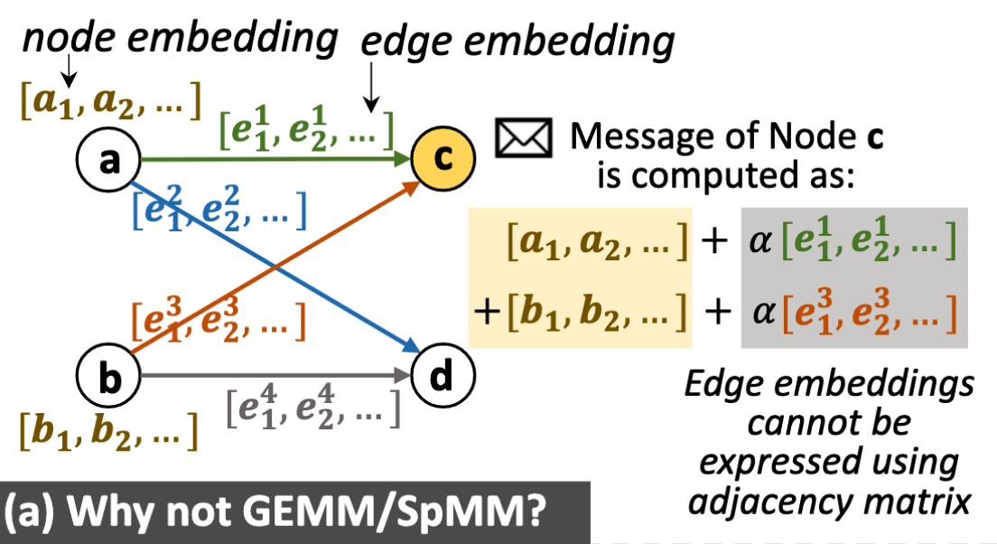
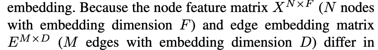
if not use edge embedding, message passing is $\phi (x_i^l)$, and it can be optimized by GEMM and SpMM.However, if use embedding, it will be $\phi (x_i^l,e_{i,j}^l)$, and the demension of node representation and edge representation is not same.
Invalid existing optimizations
SOTA I-GCN merge the same neighbor node as one node to optimize.
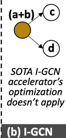
However, considering edge embedding, the $e_{ac},e_{bc}$ is not the same as $e_{bc},e_{bd}$
we cannot converge the node a and b
Non-trivial aggregation
the GEMM and SpMM use a certain pattern to optimize. However ,the compute coefficient is dynamic.
Anisotropic GNNs
such as GAT, it has a attention coefficient which is calculated by $x_i^{l},x_j^l$. and it is dynamic, which prevents GAT from being expressed as matrix multiplications to optimize.
Pre-processing
not applicable in RT application
Motivations and Innovations
Innovation:
- Explicit message passing for generality
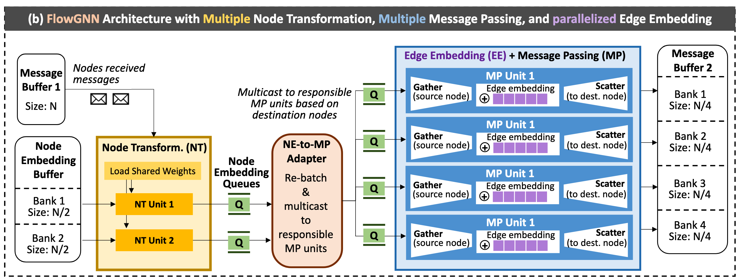
- Multi-queue multi-level parallelism for performance
GENERIC ARCHITECTURE*
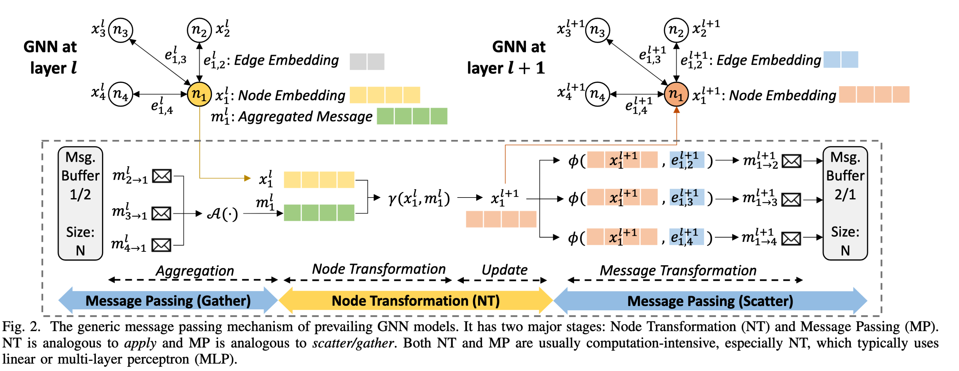
Message Passing Mechanism
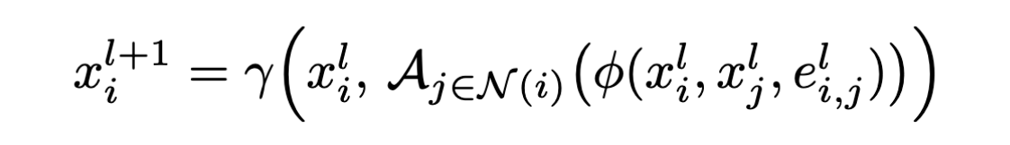
$$
\mathcal{MP scatter} \
m_{1\to 0}^{l-1}=\phi (x_1^{l-1},e_{0,1}^{l-1}) \
\mathcal{MP gather} \
m_0^l=\mathcal A(m_{1\to0}^{l-1}) \
m_1^l=\mathcal A(m_{0\to1}^{l-1},m_{2\to1}^{l-1},m_{3\to1}^{l-1}) \
\mathcal{NT} \
x_1^l=\gamma (m_1^l,x_1^{l-1})
$$
3 phases:
message passing(gather):
from message buffer get $m$, and do aggregating $A(m_{2\to1}^l, m_{3\to1}^l, m_{4\to1}^l)$.
the $\mathcal{A}(.)$ function could be sum, max, mean, std.dev.
node transformation:
$\gamma (x_1^l, m_1^l)$.
$\gamma (.)$ could be full-connected layer, MLP…
message passing(scatter):
$\phi (x_1^{l+1},e_{1,2}^{l+1})\to m_{1\to 2}^{l+1}$. Sent it to message buffer for the next layer Message passing(gather)
Baseline Dataflow Architecture
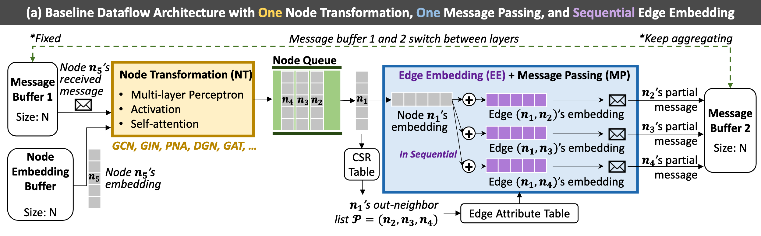
use ping-pang buffer(b => d):
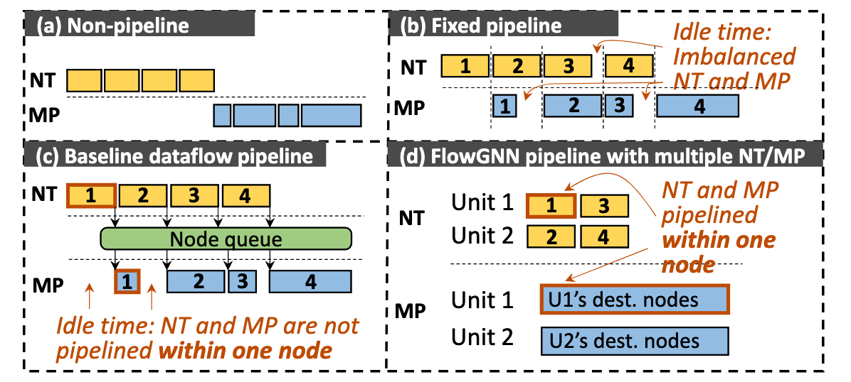
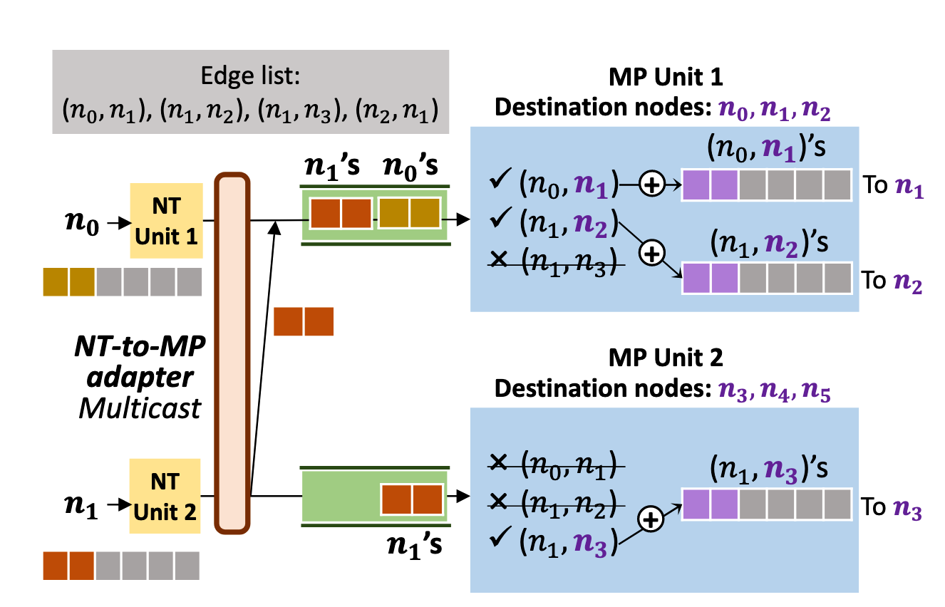
Proposed FlowGNN Architecture